Phase Demodulation using the Hilbert transform in the frequency domain


Author: Gareth Forbes Created: 30/11/09 Contact:		Downloads: PDF version

The general idea

A phase modulated signal is a type of signal which contains information in the variation of its phase, an example of a phase modulated signal, in its simplest form, is a single sine wave modulated by another sine wave, such as:

$x(t) = Acos[\Omega t+\gamma+\beta sin(\omega t+\phi)]$ (1)

Evidently phase demodulation of a signal involves reconstructing a signal such that one can characterise how the modulated signal's phase changes with time. Phase demodulation is therefore based on this simple idea of setting out to measure how the phase of the signal varies with time.

For the above simple phase modulated signal, a pragmatic approach might lead you to consider that the measurement of the phase as in fact being trivial by taking the inverse cosine of the time series $x(t)$ . This will though result in an erroneous solution.

Without going into detail, which can be proven to oneself by an interested reader, the inversion of the trigonometric function in the time domain results in an erroneous solution essentially due to the ambiguity of the trigonometric function. For instance, the cosine trigonometric function is ambiguous in that the phase angles cannot be distinguished between being in the 1st and 4th quadrant on the unit circle or similarly between the 2nd and 3rd quadrants.

However if we express the above example as a complex exponential,

$x(t) = Ae^j^{[\Omega t+\gamma+\beta sin(\omega t+\phi)]}$

then characterising the phase at any instant in time could be simply obtained by observing the angle between the real and imaginary value of the complex signal at that same instant in time.

Thus expressing a real signal in a complex form, of which the real part is the original signal, is the aim of frequency domain Hilbert transform phase demodulation. This complex signal representation is often referred to as the analytic signal.

Therefore it needs to be set about seeking how to change our real signal into its complex form.

How to implement (the maths)

By utilising Euler's formula,

$e^j^\theta = cos(\theta)+isin(\theta)$

the above simple example signal, equation (1), can be representing in its analytic form by adding the original signal with the sine of the instantaneous phase (the instantaneous phase being $\phi (t) = arg[x(t)]$ ) of the original signal multiplied by the imaginary unit 'i'. So in order to construct the analytic signal we need to find a way of transforming a cosine into a sine. It so happens that the transform for changing cosine's to sine's and visa versa is called the Hilbert transform, being:

$H[sin(t)] = -cos(t)$

$H[cos(t)] = sin(t)$

where $H$ is the Hilbert transform operator.

Nothing more needs to be discussed about the Hilbert transform itself, suffice to say that it is the technical name of the process to be used here.

We will now show a convenient way of constructing the analytic signal for our example signal with a judicious use of the Fourier transform.

If we first represent a cosine in its complex form:

$f(t) = cos(\Omega t) = \frac{e^{j \Omega t}+e^{-j \Omega t}}{2}$ (2)

Also given that the Fourier transform of a signal is:

$f(\omega) = \frac{1}{\sqrt{2\pi}}\int_{-\infty}^\infty \! f(t)e^{-j\omega t} \, dt$

Therefore the Fourier transform of (2) is:

$f(\omega) = [\delta (\omega - \Omega)+\delta (\omega + \Omega)]/2$ (3)

where $\delta$ is the Dirac delta function.

If we now set the negative frequencies of equation (3) above to zero, multiply by 2, then inverse Fourier transform we get a new function $g(t)$ , where

$g(t) = e^{j \Omega t}$

It is seen that $g(t)$ is the previously defined analytic signal of $f(t)$ . So you can see, by taking a signal into the frequency domain by Fourier transformation, setting negative frequency's to zero and doubling all positive frequency's then we have managed to add a real signal with the complex multiplied Hilbert transform of the same signal giving the so called analytic signal. It will now be shown, with application, how to implement this practically to phase demodulate a signal.

How to implement (matlab example)

(All steps can be cut and pasted into matlab's desktop window) Create a modulated signal in the same form as in equation (1)



A = 1; %magnitude

tp = 2^12; %number of time steps

omega1 = 240; %carrier freq

omega2 = 10; %modulation freq

gamma = pi/7; %phase offset

beta = 5; %modulation amplitude

t = 0:2*pi/tp:2*pi*(1-1/tp); %time vector

x = A*cos(omega1*t+gamma+beta*sin(omega2*t)); %phase modulated signal

plot(t(1:round(length(x)/omega2)),x(1:round(length(x)/omega2))) %plot modulated signal

xlim([0 t(round(length(x)/omega2))])

xlabel('time (s)')

ylabel('magnitude')

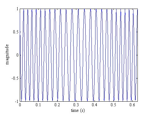
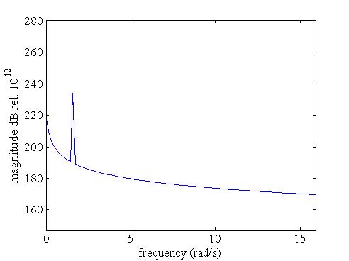
Figure 1. Time series of equation (1). Note that the phase modulation is not readily visible

Transform the signal into the frequency domain



ff = fft(x); %fourier tranform of time signal

ax = linspace(-tp/pi/4,(tp-2)/pi/4,tp); %x axis

dbf = 20*log10((abs(ff)/length(ff)*2+10E-12)/10E-12); %change spectrum into dB's

dbf = fftshift(dbf); %shift spectrum for display

plot(ax,dbf); %plot modulated signal spectrum

xlim([-tp/pi/4 tp/pi/4]) 

ylim([0 1.2*max(dbf)])

xlabel('frequency (rad/s)')

ylabel('magnitude dB rel. 10 ^{-12}')

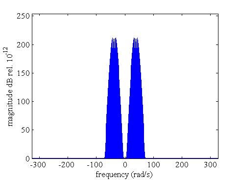
Figure 2. Spectrum of phase modulated signal as in equation (1)

Set negative frequencies to zero, and double all positive frequencies (remember not to double the zero frequency) and inverse transform back to the time domain to create the analytic signal.



gf = ff; %create dummy variable

gf(2:end) = 2*ff(2:end); %double positive freq's

gf(end/2+1:end) = 0; %set negative freq's to zero

g = ifft(gf); %transform back to time domain

dbg = 20*log10((abs(gf)/length(gf)*2+10E-12)/10E-12); %change analytic spectrum in dB's

dbg = fftshift(dbg); %shift spectrum for display

plot(ax,dbg)

xlim([-tp/pi/4 tp/pi/4])

ylim([0 1.2*max(dbg)])

xlabel('frequency (rad/s)')
ylabel('magnitude dB rel. 10^-12')

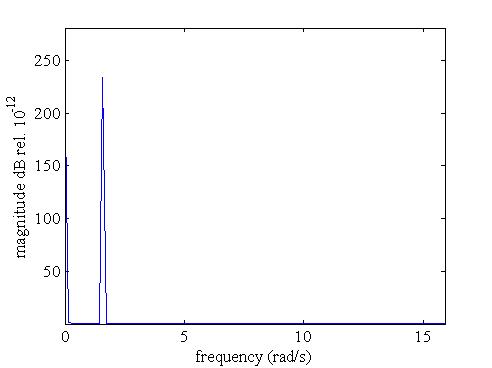
(Note the analytic signal can be created in one step with the use of the matlab command 'hilbert')

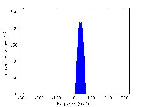
Figure 3. One sided spectrum, or spectrum of the so called analytic signal

Now calculate the instantaneous angle of the analytic signal and the unwrapped instantaneous phase of the original signal (as the matlab command angle only gives a value between 0:2pi, use the unwrap command to give the non-bound limited phase)



pha = angle(g); %instantaneous phase of analytic signal

phau = unwrap(pha); %unwrap phase

As the instantaneous phase is given by $\Omega t + \gamma + \beta sin(\omega t + \phi)$ , it can be seen the instantaneous phase increases linearly with time due to $\Omega t$ , the linear offset $\Omega t$ needs to be subtracted from the instantaneous phase to obtain the modulation term $\beta sin(\omega t + \phi)$ .

If the carrier frequency is known this can be done by multiplying the carrier frequency by the inverse of the sampling frequency and subtracting from the unwrapped instantaneous phase, or if the carrier frequency is unknown then the linear fit of the unwrapped phase will give the estimate of $\Omega t$ . This method is used here.



p = polyfit(t,phau,1); %linear fit to unwrapped phase

p(2) = phau(1); 

omega1t = polyval(p,t); 

phaus = phau - omega1t; %subtract linear offset

Now observe the spectrum of the modulating signal



mf = fft(phaus); %spectrum of phase demodulated signal

dbmf = 20*log10((abs(mf)/length(mf)*2+10E-12)/10E-12); %change spectrum to dB's

dbmf = fftshift(dbmf); %shift spectrum for display

plot(ax,dbmf); 

xlim([0 10*omega2/2/pi]) 

ylim([min(dbmf) 1.2*max(dbmf)]) 

xlabel('frequency (rad/s)') 

ylabel('magnitude dB rel. 10^-12')

Figure 4. Spectrum of the phase modulating signal with linear fit of carrier frequency

The mass line can be seen to be due to the linear fit not being able to exactly match the linear phase increase. If the actual linear phase is used then the mass line can be seen to be removed:



phaus2 = phau - omega1*t; %removal of linear phase increase if carrier freq is known

mf2 = fft(phaus2); 

dbmf2 = 20*log10((abs(mf2)/length(mf2)*2+10E-12)/10E-12); 

dbmf2 = fftshift(dbmf2); 

plot(ax,dbmf2); 

xlim([0 10*omega2/2/pi]); 

ylim([min(dbmf2) 1.2*max(dbmf2)]); 

xlabel('frequency (rad/s)'); 

ylabel('magnitude dB rel. 10^-12');

Figure 5. Spectrum of the phase modulating signal using known carrier frequency

If we now observe the phase and amplitude of the modulation signal, they are found to be very close to the actual values



gammae1 = abs(mf(1))/length(mf); 

betae1 = abs(mf(omega2+1))/length(mf)*2; 

gammae2 = abs(mf2(1))/length(mf2); 

phie1 = angle(mf(omega2+1))+pi/2; 

betae2 = abs(mf2(omega2+1))/length(mf2)*2; 

phie2 = angle(mf2(omega2+1))+pi/2;

Table 1. Actual and estimated signal parameters after demodulation

	Actual	Linear fit of phase offset	Known linear phase offset
$\beta$	5	4.970	5
$\gamma$	0.4488	0.477	0.4488
$\phi$	0	0	0

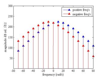
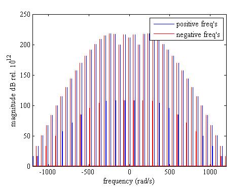
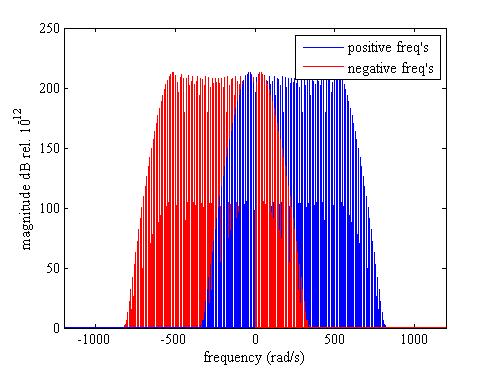
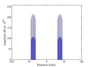
Bandwidth considerations

Some considerations on the bandwidth of both the modulating signal and the carrier frequency relationship will now be discussed. Three general rules of 'thumb' will be given for bandwidth's which will commonly result in a phase modulated signal which can be demodulated with conventional techniques.

Despite the discussion of the various bandwidth considerations that will be developed below, first and foremost the major requirement for accurate demodulation is the separation of the negative and positive frequency sidebands in the signals spectrum. This criteria is the application of the initial condition of Bedrosian's Theorem [1]. This theorem states in its most succinct form, when applied to a phase modulated signal, that the respective frequency domains of the carrier and modulating functions are non-intersecting and that the frequency of the carrier is higher than the modulating frequency for the general solution of the Hilbert transform to hold [2].

Whether this separation is present is often evident from simply viewing the spectrum, as can be seen in Figure 2 where the positive and negative frequency sideband regions are clearly separated. However when this is not evident from simply viewing the spectrum some rules of 'thumb' which can be applied to help achieve accurate demodulation will be discussed.

Fundamentally, for conventional demodulation, the maximum modulating frequency must be at least less than the carrier frequency, however this constraint alone does not provide a signal which is able to be accurately demodulated as only one set of sidebands may only be able to be used in the demodulation. We can in investigate this limitation by firstly expressing a phase modulated signal as its expanded Bessel series.

$x(t) = Acos[\Omega t + \gamma + \beta sin(\omega t + \phi)] = A\displaystyle\sum_{-\infty}^{\infty} J_n(\beta)cos[\Omega t + \gamma + n(\omega t + \phi)]$

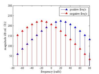
As it can be seen the spectrum of a modulated signal will have an infinite set of frequencies located at the carrier frequency plus and minus the modulating frequency. Looking at the spectrum it will have components at $\Omega \pm n\omega$ . When $\Omega=\omega$ it is seen that there will be a frequency which is wrapped around zero by the second term in the series, i.e. the second sideband, this is illustrated in Figure 6 (left).

Figure 6.(left) $\Omega=10, \omega=10, \beta=1$ . (right) $\Omega=20, \omega=10,\beta=1$

This limitation can be discussed with the introduction of a term for the ratio of carrier to modulation frequency being:

$R = \frac{\Omega}{\omega}$

It can be seen that first set of sidebands is corrupted by this frequency wrapping and that the sidebands equal or greater than the ratio $R$ will be completely corrupted by the frequency wrapping, this is shown in Figure 6, for $R=1$ and $R=2$ respectively. In general however, a ratio of $R \leq4$ is needed in order to obtain enough significant sidebands, which are not appreciably corrupted from frequencies wrapping around zero, for accurate demodulation. If an extreme case of carrier to modulating frequency ratio, of $R=1/6$ is observed as in Figure 7, then it can be seen that the entire spectrum is corrupted by the negative frequencies, and therefore demodulation of a signal such as this is not able to be achieved with this form of demodulation, and can not be accomplished with any type of conventional demodulation. Some signals with specific characteristics can however be demodulated that violate these assumptions, with the use of unconventional methods, one example of this can be found in Ref. [3].

These limitations and indeed the whole phase demodulation theory can be applied to a modulating signal which is broadband in nature. In that case these bandwidth limitations apply to the highest frequency in the modulating signal.

Figure 7. $\Omega=10, \omega=60, \beta=5$

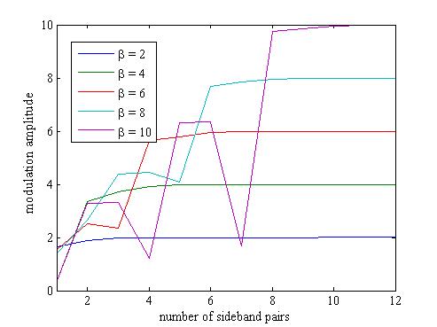
The value of $R$ such that the signal can be demodulated accurately is actually also a function of the modulation amplitude. For various modulation amplitude values, the estimate of the modulation amplitude is plotted for an increasing number of sidebands used in the demodulation. For instance you can see that for $\beta=8$ , 9 sets of side bands are needed for a less than 1% error in the amplitude estimate. For this number of sidebands to be available for use in the demodulation without wrapping around the zero frequency, a ratio of $R$ needs to be greater than 9. If this condition is not adhered to then frequency wrapping can also occur as can be seen in Figure 9 where $\beta=30$ and $R=24$ .

Two good rules of thumb that can be derived from these results, that should be adhered to for accurate demodulation are; Firstly

RULE OF THUMB 1:

$R \geq 4$

Secondly the modulation amplitude should be limited by:

RULE OF THUMB 2:

$\beta \leq R$

This now brings up the question of how many sidebands should be included to obtain an accurate demodulation without undue computation cost? The number required for any given degree of accuracy can be obtained from observation of Figure 8 however a general criteria which is often used is only including sidebands up to when any higher sidebands are less than 100 times smaller than the highest amplitude sideband. With the minimum lower limit on the number of sidebands included being 3 pairs.

So the last rule of thumb for demodulation is that the number of sidebands that should be included be greater than 3 pairs of sidebands for a modulation amplitude of less than 2.

RULE OF THUMB 3:

If $\beta \leq 2$ number of sidebands used in demodulation should be no less than 3 pairs.

Figure 8. Estimates of modulation amplitude with increasing number of sidebands used in the demodulation for different modulation amplitudes as shown

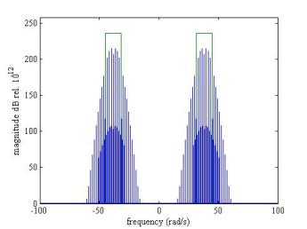
Figure 9. Wrapping due to a large modulation amplitude. $\Omega=240, \omega=10, \beta=10$

Lastly filtering should generally be done whenever the full bandwidth is not being used for demodulation, which is normally the case. The signal should be band-pass filtered around the carrier and sidebands, that are to be used in the demodulation, to avoid distortion from out of band frequencies. For example it is shown in Figure 10 the band-pass filtered spectrum for $\beta=2$ , and using 4 pairs of sidebands for demodulation, which was stated earlier as being sufficient for a modulation amplitude of $\beta \leq 2$ .

Figure 10. (left) Spectrum and overlaid band-pass filter. (right) Band-pass filtered spectrum

[1] Bedrosian, E.A. A product theorem for Hilbert Transforms Proceedings of IEEE, 1963. 51(5): p. 868-869.

[2] Cerejeiras, P., Q. Chen and U. Kahler, A necessary and sufficient condition for a Bedrosian identity. Mathematical Methods in the Applied Sciences, 2009.

[3] Forbes, G.L. and R.B. Randall, Simulation of Gas Turbine blade vibration measurement from unsteady casing wall pressure, in Acoustics 2009: Research to Consulting. 2009, Australian Acoustical Society: Adelaide.

Phase Demodulation by Gareth Forbes is licensed under a Creative Commons Attribution-Non-Commercial 2.5 Australia License.

Vibration and Acoustics Research Group, UNSW Sydney NSW 2052, Australia
Tel +61 2 9385 4093 | Fax +61 2 9663 1222 | Email mech@unsw.edu.au
Authorised by: | Privacy Statement | Copyright & Disclaimer